Modeling the behavior of short term interest rates
There are a number of ways that are used for modeling short term interest rates. These have not been covered in the PRMIA handbook, but they find a reference in one of their study guides. So just to be cautious, a bit of explanation for these is provided here in case there are questions in the exam relating to these concepts.
What should you know? Well, in all likelihood you will not be asked a question on this topic, but if you have 20 minutes, have a read and you will be slightly better prepared. Recognize the formulae for the 5 models mentioned here, and try to remember some of the differences between the no-arbitrage and equlibrium models. Or you could entirely skip this as well. I will be putting a few questions in on this subject, but will clearly mark them as unlikely.
We have seen how we expect stock prices to behave – returns being normally distributed and consequently prices distributed lognormally. If you recall, the process for the behavior of stock prices is explained as follows
[ The way stock prices work is as follows. If ΔS is the change in price, μ the returns for one time period, and σ the volatility for the same time period, then the expected change in price for the time period dt is defined as follows:

Where dt is the time (a very short period of time), and dz is the Weiner process. What we mean by ‘dz is the Weiner process’ is that dz is replaced in the above equation by a random number drawn from a standard normal distribution. This number can be randomly drawn, and in Excel we can draw a random number from a normal distribution using the formula = NORMSINV(RAND()). ]
The same process however cannot be applied to interest rates. This is because while stock prices may follow a random walk, interest rates are generally considered mean reverting. Mean reverting means they tend to come back to some long term average, and can’t increase or decrease indefinitely.
The models of short term interest rates help determine the shape of the yield curve, and option pricing on bond options. There are two broad categories of models of the short rate – Equilibrium models, and No-arbitrage models.
Equilibrium models
1. The Vasicek model
In the Vasicek model, interest rates can be modeled using the following equation:
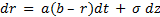
where dr is the change in the rate, a is the ‘speed of reversion’ to the mean, b is the long term mean for the rate, σ is the volatility of the rate, and dz is a weiner process. (Recall that for our practical purposes a ‘weiner process’ is nothing but a random drawing from a normal distribution). Interest rate volatility is constant at σ.
With the Vasicek model, rates will get pulled to the long term mean ‘b’ because of the first term in the formula above.
With the equation dr = a(b – r)dt + σ dz it is possible (with some more mathematics, and with known values of a, b and r) to determine the price of a zero coupon bond at any time t in the future, and thereby construct an yield curve. This yield curve will likely be different from the real one in the markets at the present time, and this divergence from reality is a big limitation of the Vasicek model. One way to overcome this limitation is to choose a, b and r in such a way that we get an yield curve close to the current yield curve, but that is often not a practical solution as such ‘fitting’ still leaves large errors.
2. The Cox, Ingersoll, and Ross model
According to the Cox, Ingersoll and Ross model, the risk neutral process for the short rate r is as follows:
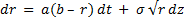
The only difference between the Vasicek model and this is that the change in the short rate is also determined by r, in the form of √r being incorporated in the formula. This has the effect of increasing the standard deviation of the rate as r goes up.
Both the Vasicek and the Cox, Ingersoll and Ross models are single factor models, dependent only upon the value of r as the single factor driving changes to short rates.
No-arbitrage models
The yield curves predicted by the equilibrium models are generally different from what are being observed at the current time in the markets. It is possible to tweak the values of a and b to arrive to a close fit, but still large errors often remain. This problem is solved by using the current term structure as an input into the model so the model ends up being exactly consistent with the today’s term structure.
3. The Ho-Lee model
Under the Ho-Lee model,
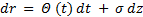
All variables have their usual meaning, but Θ(t) is a function of time selected to fit the initial term structure. Θ(t) can be analytically calculated using a formula (probably not relevant for the exam), suffice it to say it is a function time t.
4. The Hull White model
The Hull White model is an extension of the Vasicek model with the difference that it can be made to fit the current term structure.
Under the Hull White model:

or
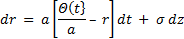
The mean reversion happens at the rate a. At time t, the rate shows a mean reversion to Θ(t)/a at rate a.
5. The Black-Derman-Toy model
Under the Ho-Lee and Hull-White models, interest rates can become negative. The BDT model allows only positive interest rates, and is as follows:
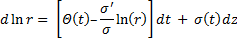
Where Θ(t) is a function of time, and σ is the volatility of the short rate.
The models of short rates are used to price fixed income derivatives and bonds.