This article attempts to provide an intuitive understanding of what PCA is, and what it can do. PRMIA has been asking questions on PCA, but the way the subject is presented in the Handbook is not appropriate for someone who has not studied it before in the classroom. This article aims to provide an intuitive understanding of what PCA is so you can approach the material in the handbook with confidence.
But before we even start on Principal Component Analysis, make sure you have read the tutorial on Eigenvectors et al here. Otherwise much of this is not going to make any sense.
The problem with too many variables
The problem we are trying to solve with PCA is that when we are trying to look for relationships in data, there may sometimes be too many variables for doing anything meaningful. What PCA allows us to do is to replace a large number of variables with much fewer ‘artificial’ variables that effectively represent the same data. These artificial variables are called principal components. So you might have a hundred variables in the original data set, and you may be able to replace them with just two or three mathematically constructed artificial variables that explain the data just about as well as the original data set. Now these artificial variables themselves are built mathematically (and I will explain that part in a bit), and are linear combinations of the underlying original variables. These new artificial variables, or principal components, may or may not be capable of any intuitive human interpretation. Sometimes they may just be combinations of the underlying variables in a way that make no logical sense, and sometimes they do provide a better conceptual understanding of the underlying data (as fortunately they do in the analysis of interest rates and for many other applications as well).
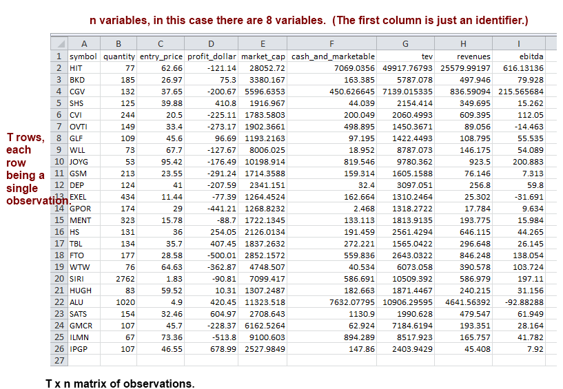
Let us take an example. Imagine a stock analyst who is looking at the returns from a large number of stocks. There are many variables he/she is looking at for the companies he is analyzing, in fact dozens of them. He has all of his data in a large spreadsheet, where each row contains a single observation (for different quarters, months, years or whatever way the data is organized). The columns read something like the list below. The data can be thought of as a T x n matrix, where T is the rows, with each row being an observation at a point in time, and n being the number of data fields.
- Company name
- PE ratio (Price Earnings)
- NTM earnings (Next 12 months consensus earnings)
- Revenue
- Debt
- EPS (Earning per share)
- EBITDA (Earnings before interest, tax, depreciation and amortization)
- LQ Earnings (Last quarter’s earnings)
- Short Ratio
- Beta
- Cash flow
…etc up to column n.
If the analyst wants to analyze the relationship of the above variables to returns, it is not an easy task as the number of variables involved is not manageable. Of course, many of these variables are related to each other, and are highly correlated. For example, if revenues are high, EBITDA will be high. If EBITDA is high, Net Income will be high too, and if Net Income is high, so will be the EPS etc. Similar linkages and correlations can be seen with cash flows, LQ earnings etc. In other words, this represents a highly correlated system.
So what we can do with this data is to reduce the number of variables by condensing some of the correlated variables together into one single representation (or an artificial variable) called a ‘principal component’. How good is this principal component as a representation of the underlying data it represents? That question is answered by calculating the extent of variation in the original data that is captured by the principal component. (All these calculations, including how principal components are identified, are explained later in this article. For the moment let us just go along to understand conceptually what PCA is.) The number of principal components that can be identified for any dataset is equal to the number of the variables in the dataset. But if one had to use all the principal components, it would not be very helpful because the complexity of the data is not reduced at all, and in fact is amplified because we are replacing natural variables with artificial ones that may not have a logical interpretation. However, the advantage that identifying principal components brings is that we can decide which principal components to use and which to discard. Each principal component accounts for a part of the total variation that the original dataset had. We pick the top 2 or 3 (or n) principal components so we have a satisfactory proportion of the variation in the original dataset.
You might be wondering – what does ‘variation’ mean, in the sense of total variation and the explained variation that I just mentioned. So think of the data set as a scatterplot. If we had two variables, think about how they would look when plotted on a scatter plot. If we had three variables, try to visualize a three dimensional plane and how the data points would look – like a cloud kind of clustering together a little bit (or not) depending upon how correlated the system is. The ‘spread’ of this cloud is really the ‘variation’ contained in the data set. This can be measured in the form of variance, with each of the n columns having a variance. When all the principal components have been calculated, each of the principal components has a variance. Fortunately, the simple summation of the variance of the individual original variables is equal to the summation of the variances of the principal components. But it is distributed differently. We arrange the principal components in descending order of the variance each of them explains, take the top few principal components, add up their variance, and compare it to the total variance to determine how much of the variance is accounted for. If we have enough to meet our needs, we stop there, otherwise we can pick the next principal component in our analysis too. In finance, PCA is often performed for interest rates, and generally the top three components account for nearly 99% of the variance allowing us to use the just those three instead of the underlying 50-100 variables that arise from the various maturities (1 day to 30 years, or more).
PCA in practice
This is how the drill works:
- PCA begins with the covariance (or correlation) matrix. First, we calculate the covariance of all the original variables and create the covariance matrix.
- For this covariance (or correlation) matrix, we now calculate the eigenvectors and eigenvalues. (This can be done using statistical packages, and perhaps also some commercial Excel add-ins.)
- Every eigenvector would be a column vector with as many elements as the number of variables in the original dataset. Thus if we had an initial dataset of the size T x n (recall: rows are the observations, columns represent variables, therefore we have T observations of n variables), the covariance matrix would be of the size n x n, and each of the eigenvectors will be n x 1.
- The eigenvalues for each of the eigenvectors represent the amount of variance that the given eigenvector accounts for. We arrange the eigenvectors in decreasing order of the eigenvalues, and pick the top 2, 3 or as many eigenvalues that we are interested in depending upon how much variance we want to capture in our model. If we include all the eigenvectors, then we would have captured all the variance but this would not give us any advantage over our initial data.
- In a simplistic way, that is about all that there is to PCA. If you are reading the above for the first time, I would understand if it all gobbledygook. But no worries, we are going to go through an example to illustrate exactly how all of the above is done.
Example:
Let us consider the following data that explains the above. This is just a lot of data, typical stuff of the kind that you might encounter at work. Let us assume that this is data relating to stocks, with the symbols appearing in column A, and various variables relating to the symbol on the right. What we want to do is to perform PCA on this data and reduce the number of variables from 8 to something more manageable. We believe this can be done because if we look at the variables, some are obviously quite closely related. Higher revenues likely mean a higher EBITDA, and a higher EBITDA probably means a higher tev (total enterprise value). Similarly, a higher price (col C) probably means a higher market cap too – though of course we can not be sure unless we analyze the data. But it does appear that the data is related together in a way that we can represent all of this fairly successfully using just a few ‘artificial variables’, or principal components. Let us see how we can do that.
Based on the above, we can calculate the correlation matrix or the covariance matrix – either manually, or in one easy step using Excel’s data analysis feature.
The problem of scale – (ie, when to use the correlation matrix and when the covariance matrix?)
Let us get this question out of the way first. Consider two variables for which the units of measure differ significantly in terms of scale. For example, if one of the variables is in dollars and another in millions of dollars, then the scale of the variables will affect the covariance. You will find that the covariance will be significantly affected by the variable that has larger numerical quantities. The variable with the smaller numbers – even though this may be the more important number – will be overwhelmed by the other larger numbers in what it contributes to the covariance. One way to overcome this problem is to normalize (or standardize) the values by subtracting the mean and dividing by standard deviation (ie, obtain the z-score, equal to (x – μ)/σ)) and replacing all observations by such z-scores.
We can then use this normalized set of observations to perform further analysis because now everything will be expressed on a standard unitless scale in a way that the mean is zero and standard deviation is 1 for both sets of observations. Now if for this set of normalized observations you will find that the correlation and covariance are identical. Why? Think for a minute about the conceptual difference between correlation and covariance. Covariance is in the units of both the variables. In a case where observations have been normalized, they do not have any units already. So you end up with a unitless covariance which is nothing but correlation. Formulaically, correlation is covariance divided by the standard deviations of the two variables. In the case where the observations have been normalized, the standard deviation of both the variable is 1 and dividing covariance by 1 leaves us with the same number. In other words, correlation is really nothing but covariance normalized to a standard scale.
Because covariance includes the units of both the variables, it is affected by the scale. Basing PCA on a correlation matrix is identical to using standardized variables. Therefore in situations where scale is important and varies a great deal between the variables, correlation matrices may be preferable. In other cases where the units are the same and the scale does not vary widely, covariance matrices would do just fine. If we run PCA on the same data once using a correlation matrix and another time using a covariance matrix, the results will not be identical. Which one to use may ultimately be a question of judgment for the analyst.
In this case, we decide to proceed with the correlation matrix, though we could well have used the covariance matrix as all the variables are in dollars. However, for the mechanics of calculating the principal components that I am trying to demonstrate, this does not matter – so we will proceed with the correlation matrix.
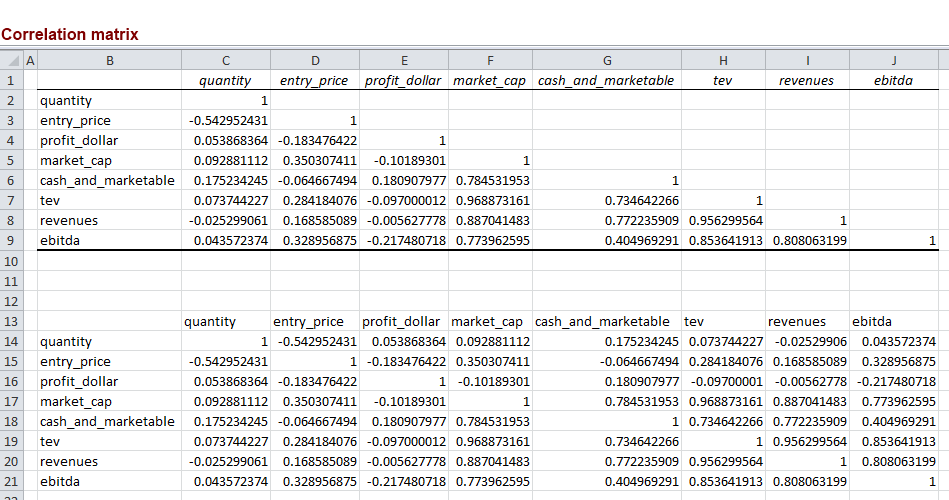
The correlation matrix appears as follows. The top part is what the Excel output looks like (Data Analysis, correlation. If you don’t have Data Analysis available in your version of Excel, that is probably because you haven’t yet installed the data analysis plug in. Search Google on how to do that). The lower part is merely the same thing with the items above the upper diagonal filled in. And for this correlation matrix, there will be n eigenvectors. It is acceptable to put all the column vectors for the eigenvectors in one big n x n matrix too (which is how you will find it in some of the textbooks, and also below).
The eigenvectors multiplied by the underlying variables represent the principal components. Thus if an eigenvector is say [0.25,0.23,0.22,0.30,0.40]-1, and the 5 variables in our analysis are v1, v2, v3, v4 and v5, then the principal component represented by that eigenvector is = 0.25v1 + 0.23v2 + 0.22v3 + 0.30v4 + 0.40v5. The other principal components are similarly calculated using the other eigenvectors.
The eigenvalues for each of the eigenvectors represent the proportion of variation captured by that eigenvector. The total variation is given by the sum of all the eigenvectors. So if the eigenvalue for a principal component is 2.5 and the total of all eigenvalues is 5, then this particular principal component captures 50% of the variation.
We decide how many principal components to keep based upon the amount of variation they account for. For example, we may select all principal components above a certain threshold of contribution to accounting for variation, or all principal components whose eigenvectors have an eigenvalue greater than 1.
We can now represent the original variables as a function of the principal components – each original variable is equal to a linear combination of the principal components
Calculating eigenvalues and eigenvectors
There is no easy way I know of that can help us calculate eigenvalues and eigenvectors in Excel. For our hypothetical example, the eigenvectors and the eigenvalues are given below. (These were calculated in a different statistical package (R, which is free to use, and can be downloaded from www.r-project.org). The R commands to use for this specific example are provided at the bottom of this write-up.).

What is ‘Total variance’ that we talk about?
This was explained before, but we can now talk about this a bit more concretely. The total variance in the data set is nothing but the mathematical aggregation of the variance of each of the variables. If the observations have been normalized, then the variance of each of the variables will be 1, and therefore the total variance will be 1 x n = n, where n is the number of variables. Once principal components have been computed, there will be a total of n principal components for n variables. The important thing to note is that the total of the variances of the principal components will be equal to the total variance of the observations. This allows us to pick the more relevant principal components by picking the ones with the most variance and ignoring the ones with the smaller variances, and still be able to cover most of the variation in the data set.
Notice that the total of the eigenvalues is 8 – which is the same as the number of variables. Because we effectively normalized the variables by using the correlation matrix, the total of our eigenvalues is 8 which is the sum of the individual normalized variances (=1) of each of the eight variables. (If we had used the covariance matrix, the eigenvalues would have added to whatever the sum of the variances of each individual variable would have been.)
We also see that just the first 2 principal components account for nearly 75% of the variance. If we are comfortable with the simplicity that 2 variables offer instead of 8 at a cost of losing 25% of the variation in the data, we will use 2 principal components. If not, we can extend our model to include the third principal component which brings the total variance accounted for to nearly 88%.
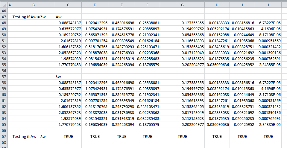
Is Aw = λw?
Do our eigenvalues and eigenvectors satisfy Aw = λw, where w is the eigenvector, A is a square matrix, w is a vector and λ is a constant? Let us test that. In this case, A is our correlation matrix, w is the eigenvector and λ is the eigenvalue. We find this relationship to be true for all eigenvectors.
Constructing principal components from eigenvectors
We derive the principal components from the eigenvectors as follows.
PC1 = -0.02070*quantity -0.14822*entry_price 0.04413*profit_dollar -0.47031*market_cap -0.37456*cash_and_marketable -0.47874*tev -0.46308*revenues -0.41295*ebitda
PC2 = 0.60642*quantity -0.63912*entry_price 0.33582*profit_dollar 0.00458*market_cap 0.30794*cash_and_marketable 0.01122*tev 0.04846*revenues -0.11699*ebitda
PC3 = -0.44257*quantity 0.16687*entry_price 0.81688*profit_dollar -0.00946*market_cap 0.23303*cash_and_marketable -0.03034*tev 0.08786*revenues -0.21437*ebitda
And so on.
How do we use the principal components for further analysis? For any observation, we set up a routine to calculate the principal component equivalent and use that instead of the original variables – whether for regression, or any other kind of analysis. So PCA is merely a means to an end – it does not give you an ‘answer’ that you can use right away.
Are my principal components orthogonal?
We can verify this quite easily by taking any two principal components and calculating their dot product (see the tutorial on eigenvectors and eigenvalues referred to at the beginning of this tutorial). We find that this indeed is the case. If you would like to test it yourself, the Excel spreadsheet used in this tutorial is available from a link at the bottom of this article.
Is my correlation matrix positive definite?
A matrix is positive definite if all its eigenvalues are greater than zero, which indeed is the case for the example above.
Interpreting principal components
We look at the coefficients assigned to each of the principal components, and try to see if there is a common thread between the factors (in this case, quantity, entry_price, profit_dollar etc are the ‘factors’). The common thread could be an underlying common economic cause, or other explanation that makes them similar. In our hypothetical example, we find that the first principal component is heavily “loaded” on the last 5 factors. The second principal component is similarly “loaded” on the first three, and also a bit on the fifth one. (You can see this by examining the eigenvectors for the respective principal component.)
In the case of interest rates, by looking at how the principal components are constructed, we find that the first 3 principal components are called the trend, the tilt and the curvature components.
You can download the Excel file from which the above screenshots were taken here
That is all for PCA folks! Hope the above made sense and is helpful. Feel free to reach out to me by email if you think something above is not correct or can be improved, or if you just have a comment or a question.
————————–
Notes – calculating eigenvalues and eigenvectors in R:
# Below appears the R commands, that you can cut and paste directly on the R console
# First, we create the matrix “t” in R as follows – this uses the same numbers as in the Excel:

t <- matrix(data = c(
1, -0.542952431442194, 0.0538683636417128, 0.092881111887128, 0.175234245236797, 0.0737442268730075, -0.0252990610100093, 0.0435723741613164,
-0.542952431442194, 1, -0.183476421520677, 0.350307411119932, -0.0646674944921761, 0.284184075846036, 0.168585089119576, 0.328956875259816,
0.0538683636417128, -0.183476421520677, 1, -0.101893010169862, 0.180907977203587, -0.0970000119510433, -0.00562777781643539, -0.217480718025955,
0.092881111887128, 0.350307411119932, -0.101893010169862, 1, 0.784531952961134, 0.968873161130009, 0.887041483244711, 0.773962594956624,
0.175234245236797, -0.0646674944921761, 0.180907977203587, 0.784531952961134, 1, 0.734642266097147, 0.772235909124476, 0.404969290979045,
0.0737442268730075, 0.284184075846036, -0.0970000119510433, 0.968873161130009, 0.734642266097147, 1, 0.956299563903862, 0.853641912798971,
-0.0252990610100093, 0.168585089119576, -0.00562777781643539, 0.887041483244711, 0.772235909124476, 0.956299563903862, 1, 0.808063198919785,
0.0435723741613164, 0.328956875259816, -0.217480718025955, 0.773962594956624, 0.404969290979045, 0.853641912798971, 0.808063198919785, 1),
nrow=8)

# Second, we get the eigenvalues and eigenvectors and store them in a variable, say “myeigen”

myeigen <- eigen(t)

# You can print myeigen on screen to see the eigenvalues and eigenvectors, and they are listed in descending order of the eigenvalues.
# Also, the way R provides you the output is such that the eigenvalues and eigenvectors are lined up correctly.

myeigen

# We can see individual eigenvalues as follows, where you can use any number instead of 1 to get the respective eigenvalue.

myeigen$values[1]

# Similarly we can see the individual eigenvectors as follows, where you can use any number instead of 1 to get the respective eigenvector.

myeigen$vectors[,1]

# We can also check if Aw = lambda x w.  We get Aw as follows

t %*% as.matrix(myeigen$vectors[,1])

# We multiply the eigenvalue with the eigenvector to get the same matrix as above, showing that the eigenvalue and eigenvectors
# are indeed correct.

myeigen$values[1] * as.matrix(myeigen$vectors[,1])