This is a very brief article, perhaps unjust given what it covers. I have tried to keep it very short, so as to be a practical reference to key statistical terms that are used throughout risk management. This covers standard deviation, variance, covariance, correlation, regression and the famous ‘square root of time’ rule. The PRMIA handbook has more stuff but this covers the key things you must know – almost by heart!
Returns, volatility, correlation and regression analysis are basic statistical tools that are used throughout finance. It is important to have a good intuitive understanding of all these concepts and how they tie together. While this brief tutorial is not a replacement for your statistics text book, I have tried to capture all the key relationships and formulae you are going to need for the PRMIA exam.
Mean:
Mean is just the average, and is given by the formula:

(I will not explain what n and x-bar are, the usual conventions have been followed.)
Among other things, mean is used to describe asset returns. If S2 be the price of an asset at time 2, and S1 be the price at time 1, then
Returns = ![]()
Compounded returns = ![]() where LN is the natural logarithm.
where LN is the natural logarithm.
Standard deviation and Variance
Standard deviation is a measure of the variability of a set of data. If x be the mean of a set of data, then standard deviation measures how much variation there is in individual observations around this mean. A natural reaction to measure variability would be to find the difference between each observation and the mean, and divide by the number of observations to find out how much does each observation differ from the mean ‘on average’. Unfortunately intuition does not serve us well here as the summation of individual differences from the mean is zero.
In other words, this doesn’t work because:

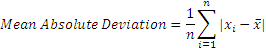
So this doesn’t help us much. Again, next natural response would be to take the absolute value of the differences, and take an average. While this resulting number (called mean absolute deviation) is a little bit more useful, it is not really useful for further analysis or for being included in other advance calculations as the resultant is erratic, unpredictable and not much further math can be done on it.
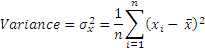
The final solution is to square the differences from the mean, and take a square root. This is a mathematical operation that is predictable and gives us a much better sense of how ‘variable’ a number is. The result is standard deviation, whose square is variance.
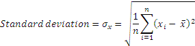
The term ‘volatility’ refers to standard deviation. Watch out for questions that refer to volatility and provide variances. Also remember that volatility is usually measured in years, so unless specifically mentioned in a question (eg volatility per day), volatility refers to annual standard deviation.
Standard deviation is expressed in the units of the variable, and variance in the square of the variable’s units. Also, note that standard deviation (or variance) is expressed in terms of expected variability per unit of time, ie, volatility could be daily, monthly, annualized, or any other time period that is relevant. The smaller the time period, the lesser is the volatility that we are exposed to, and volatility would be greater for longer time periods.
The square root of time rule
If the returns of two assets in a portfolio are independent, their variances can be added to get the combined variance for the portfolio. The standard deviation of a group of uncorrelated assets therefore is the square root of the sum of their variances. This property can be used to calculate the standard deviation for any time period provided we assume that returns across time periods are independent of each other.
The square root of time rule is often used to convert standard deviation from a given time period to the standard deviation for another time period. A common application is converting a 1-day volatility to a 10-day volatility (and by extension, converting a 1-day VaR estimate to a 10-day VaR estimate).
If we know the standard deviation for a given time period, say ‘old time period’ and need to convert it to a ‘new time period’, we can do so using the formula:

For example, if we know the 1-month standard deviation to be 6%, then the annualized standard deviation is = 6% x √12/1 = 20.78%.
Covariance
Covariance is the extent to which two variables tend to vary together. For two variables x and y, it is calculated as follows:

Note the similarity between the formula for covariance and variance. Variance is nothing but the covar of the variable with itself. Covariance is in the units of both the x variable and the y variable, therefore representing a number that is not intuitively understandable.
Interpreting covariance: A covariance of zero implies that the variables do not have a linear relationship. A positive covariance means that they rise and fall together, and a negative covariance means that when one rises, the other falls. The result for covariance is sensitive to the units used for each of the variables. If for example, x is a variable expressed in dollars, and we change it to be in millions of dollars, we will see covariance fall numerically though nothing would have changed in an economic sense.
Also note that independent variables will have zero covariance, but zero covariance does not imply independent variables except in a linear sense – this distinction is important. Covariance only measures linear relationships. If the relationship between two dependent variables is non-linear, it may or may not produce an appropriate covariance number.
Correlation
Correlation is nothing but covariance normalized. Since covariance is in the units of both the variables, we can strip the units by dividing by the standard deviations of both the variables. The resulting number is the correlation, is a number independent of the units of the two variables, and lies between +1 and -1.
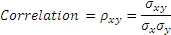
As noted for covariance, a zero correlation may hide a non-linear relationship!
Regression analysis
In simple univariate regression, we consider the simple linear relationship between two variables. If x be the independent variable and y the dependent one, then we can express the relationship between the two as:

where ϵ is the ‘error’ term, not in the sense of a mathematical error, but in the sense that our estimate would differ from the actual observed value by some unknown quantity reflecting the fact that our regression estimates are not perfect. There are other factors at play as well that we either do not know about, or are not included in our linear estimation.
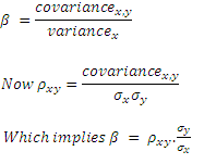
The values of α and β are estimated in a way as to minimize the squares of the ϵ variable. This is called the method of ordinary least squares.
α and β are constants, and the parameter β is known as the regression coefficient. The sign of beta is the same as that for the correlation constant between x and y. α is the intercept and β is the slope of the regression line.
Given a set of values for x and y, α and β can be estimated using the SLOPE and INTERCEPT functions in Excel.
Regression and CAPM
There is a great deal of similarity between the regression model and CAPM – in fact the CAPM is very similar to a univariate regression model where the dependent variable is the price of the stock, and the independent variable is the general market, as represented by an index. The beta in this case measures the sensitivity of the share price to movements in the market.
We take the example of the stock price for Novartis on the NYSE and regress it against the S&P500, which is a broad based market index. (The daily data was obtained from Yahoo! Finance.) Refer to this spreadsheet to see the exact workings for the regression.
The coefficient of determination: R2
The coefficient of determination helps us evaluate how good the ‘fit’ of the regression model is. It is equal to the square of the correlation coefficient, and explains how much of the squared deviations from the mean are ‘explained’. R-square is easily calculated as the square of the correlation coefficient.