This is a brief article on default correlations – what it means, and how to interpret it. To keep things simple, let us consider only two securities– A and B. Let us look at how default correlations are calculated, and then try to think about how to intuitively interpret a given default correlation number between two securities.
The question I am trying to address is something like this: when we say that the default correlation between A and B is 0.4, for example, what does it really mean? Does it mean that A and B will default together 40% of the time? Or does it mean that 40% of the defaults in either are “explained” by a default in the other? Or does it mean something completely different?
Let us get the math out of the way first so we feel confident about the mechanics before going on to looking at an intuitive understanding. Let us look at how default correlations are calculated.
Default for any security is a binary event – the security either defaults, or it does not. In other words, we can denote default by a 0, and survival by a 1. This way of representing default or survival is also correct as that represents the value of $1 of a security after the period under consideration. With this representation, calculating default correlations between the securities becomes a trivial task as shown below in three cases. What you see below are three scenarios with 20 observations each. (of course, in real life, there is only one realized observation. Once time has passed, the security will either have defaulted or not. We don’t know in advance what that realized observation will be. Consider each of the observations below as having been the outcome of the passage of time on the default or survival of our two securities in 20 identical but parallel universes – a concept that might be quite easy to think about if you grew up watching the original Star Trek).
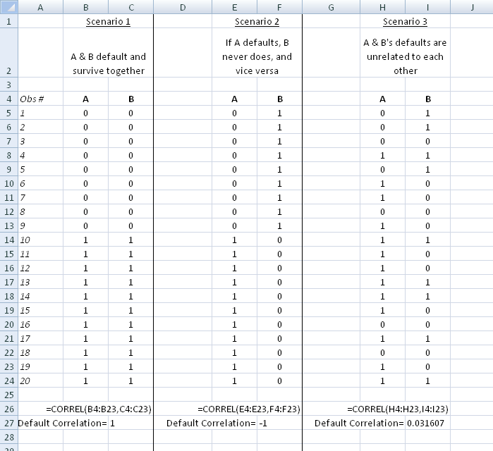
So the first scenario is one where the securities survive or default in lockstep with each other, ie, when one defaults, the other one does too, and also vice-versa. The second scenario represents the other extreme where survival by one certainly implies the other will default, or the other way round. These are the two extreme, or limiting cases, and are useful as they quite easily illustrate what default correlations of +1 and -1 mean.
The calculation of the correlation itself is done using the Excel formula ‘CORREL’, which I have illustrated in the graphic above. The third scenario represents a situation where the defaults of the two securities are completely random, and happen regardless of what happens to the other security. In such a case, the default correlation is zero, or very close to that in the hypothetical scenario described above.
An easier way to think about this is using Venn diagrams. The three cases above are depicted below. Each circle represents the marginal probability of the default of the individual securities (note: by ‘marginal probabilities’ I mean the standalone probability of default of the security regardless of the default or otherwise of the other security). Their intersecting areas represent the space where both the securities default together. It is the size of this area that is determined by the default correlation.
The way default correlation works is that the larger the default correlation, the greater is this area, or the greater is the overlap between the two circles. In other words, what default correlation allows us to do is to establish the size of this intersecting common area of joint default given known marginal probabilities.
If we were to think of the marginal probability of default of security A to be P(A), and that of security B to be P(B), then the relationship between the intersecting area (P(A⋂B)) and the default correlation is given by the following relationship:

or P(A⋂B)=Default Correlation of A&B*√((P(A)(1-P(A) ) )(P(B)(1-P(B) ) ) )+ P(A)P(B)
It is easy to see that in a situation where the Default Correlation of A & B = 0, ie, the defaults are independent, the combined probability of default is P(A)*P(B), exactly what we would intuitively expect. For example, if Security A is an Indian government bond denominated in Indian Rupees with a default probability of 1%, and Security B is a Greek bond denominated in Euros with a default probability of 6% (over identical time periods, say 10 years) and both are independent of each other (ie default correlation=0), then the probability of both of them defaulting is 1% x 6%. The formula above gives us the same result.
Now let us consider the other extreme case where default correlation is equal to 1 . This means that the securities behave in an identical fashion, ie when one defaults, the other does too, and when one survives, so does the other. Just to keep things simple and to illustrate the principle, let us also assume P(A) = P(B) = p. In such a case:
P(A⋂B)=+1*√(p(1-p ) )(p(1-p ) ) )+ p*p
= p(1-p) + p^2
= p – p^2 + p^2
= p.
Exactly what we would expect!
Now let us think of the final case where default correlation = -1, ie where default by one means the other survives and vice-versa.
In such a case, we know that the probability of joint default of the two securities will be zero, as the circles will never overlap. Let us calculate this with the formula:
P(A⋂B)=-1*√(p(1-p ) )(p(1-p ) ) )+ p*p = -p(1-p) + p^2 = – p + p^2 + p^2 = -p + 2p^2.
But –p + 2p^2 is not zero always. Why? We do know intuitively that P(A⋂B) in this case is zero. So why did our formula not evaluate to zero? The reason for this is that P(A⋂B) is affected not just by the default correlation, but also by P(A) and P(B), which in our cases we have assumed to be identical to ‘p’.
Now let us look at our formula again:
P(A⋂B)=Default Correlation of A&B*√((P(A)(1-P(A) ) )(P(B)(1-P(B) ) ) )+ P(A)P(B)
Just to make it easier to read, let us use Ψ (I would have preferred to use ρ, but it looks very much like p and can only cause confusion) to denote the default correlation, and let us also assume P(A) = P(B) = p.
∴ P(A⋂B)= Ψ *√(p(1-p ) )(p(1-p ) ) )+ p*p
= Ψ p(1-p) + p^2
= Ψ p + p^2(1- Ψ)
This means the intersecting area of the two circles is driven by both the default correlation and also p. Since P(A⋂B) is a probability, it cannot be less than 0 or greater than 1. This means that the expression Ψ p + p^2(1- Ψ) must always be greater than or equal to zero, and less than or equal to 1. Now given that p (probability of default) can be any number, the values Ψ can possibly take will be limited to the range that keeps the expression Ψ p + p^2(1- Ψ) between 0 and 1. In other words, the default correlation will not be able to vary all the way from -1 to +1.
To explain this, consider p, or the probability of default to be 20%. In such a case, P(A⋂B) = Ψ p + p^2(1- Ψ) = 0.2 Ψ + 0.04 – 0.04 Ψ = 0.16 Ψ + 0.04. For the expression 0.16 Ψ + 0.04 to never be less than 0, Ψ can never be less than -0.25. In other words, for a probability of default of 20%, the lowest the default correlation can get to is -0.25. Anything lower than that would be an absurdity. In fact, it is quite easy to show that for Ψ p + p^2(1- Ψ) >0, Ψ would need to be greater than p/(1-p). Of course, there is no such limit on the positive side. Now a probability of default of 20% is actually quite high. Since the default correlation will need to be greater than p/(1-p), it is easy to see that for real world probabilities of default (in the 0% – 3% to 4% range), the default correlation is very difficult to get negative. The lowest it gets to is about zero or thereabouts.
Therefore you will mostly encounter positive default correlations and negative default correlations are quite rare, and finding securities that are perfectly negatively correlated when it comes to default is quite rare.
Now let us take a quick look at the relationship between default correlation and the probability of joint default of two securities, the original question that we started with.
P(A⋂B) = Ψ p + p^2(1- Ψ) … … … (Equation 1)
P(A⋂B) = Ψ p + p^2- Ψp^2
P(A⋂B) = Ψ (p – p^2)+ p^2
Or, Ψ = (P(A⋂B) – p^2 ) / (p – p^2)
This is the relationship between the probability of joint default of two securities and their default correlation. Using equation 1 above, we can generally say that an increase in the default correlation increases the intersecting area in our Venn diagram where both securities default, and the exact numerical value of that area will also be driven by p, the marginal probabilities of default of the two securities.
If you have followed all of the above, that is hopefully about all you need to know about default correlation for the PRMIA exam. You will need to remember the formula for calculating the joint probability of default using p and the default correlation for numerical questions.