This article covers how Marginal and Component VaRs are calculated.  We follow up (in a separate article) with a real life example of how VaR, MVaR, undiversified VaR, Component VaR are calculated – based on actual price data pulled from Quandl, an open source market data website.

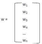
Imagine i assets in the portfolio, each with a weight of w_i.

Just another way of saying that the sum of weights equals one. The weights can be represented as a column matrix, w, as below:

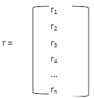
Also assume that V_i represents the dollar value of the i-th asset in the portfolio, and V, or V_p, is total portfolio value in dollars.  Now assume r_i is the return on asset i for period t, and is represented as a column vector of returns.

Portfolio returns can now be calculated as w^Tr, where w^T is the transpose of w.  In other words:

We also know that if V is the covariance matrix for the portfolio, then . Where σ_p is the portfolio variance.  For more on how we get this, and how the matrix math works, read the article on portfolio variance also posted in the tutorials.

Calculating portfolio VaR

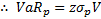
Since we know the portfolio standard deviation, VaR is easy to calculate as a product of the standard deviation and the z-score from the normal distribution for the confidence level we seek. (eg, at 95% confidence, or if α = 5%, then =NORMSINV(0.95) in Excel gives us the value for z).

Note that this is VaR as a percentage. To calculate the dollar VaR, this will need to be multiplied by the value V of the portfolio.

 – in dollars.

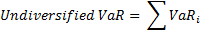
Undiversified VaR

The VaR calculation above takes into account the correlations between the assets in the portfolio. Undiversified VaR is VaR calculated as a summation of the VaRs of each individual asset. Undiversified VaR is therefore generally much larger than regular diversified VaR.

Marginal VaR for asset i

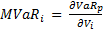
Marginal VaR for an asset i in the portfolio is the change in VaR caused when an additional $1 of the asset is added to the portfolio.

Mathematically, if V_i is the value of the i-th asset, then MVaR_i can be calculated as the derivative of VaR with respect to V_i.  Or:

We know what VaR_p is (=zσ_pV), and V_i can be written as V_pw_i, so substituting we get:

 —–Equation 1

Now we know that

or 

Differentiating this wrt w, we get

The i-th component of this is calculated as follows (more of the math is explained in Chapter 3, Vol III Book 3 of the PRMIA Handbook):

Substituting this in Equation 1 (in the last term), we get:

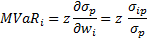———Equation 2

Even if you do not understand the calculus, that is okay so long as you know the above result and can apply it to a numerical question.

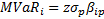
MVaR can also be expressed in terms of correlation (as opposed to covariance), and beta by taking advantage of the following relationships:

Substituting these appropriately, we get:

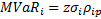———Equation 3

and 

————-Equation 4

Try to remember all the above equations numbered 1 to 4 above to prepare for any numerical questions relating to MVaR.

Calculating beta

We can also calculate the beta of the individual assets in the portfolio, which is the sensitivity of the returns between the i-th asset to portfolio returns.

Component VaR (CVaR)

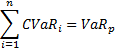
Component VaR for the i-th asset is nothing but the product of Marginal VaR and the value of the i-th asset. Component VaR has the useful property that it adds up to the dollar VaR of the portfolio, that makes life very easy from a risk disaggregation perspective.

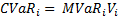
And remember that CVaR totals to VaR.